
Neural Sum-of-Squares: Certifying Polynomial Nonnegativity with Transformers
Published:
This post accompanies our ICLR 2026 paper: Neural Sum-of-Squares: Certifying the Nonnegativity of Polynomials with Transformers
Many problems in control, robotics, and optimization reduce to proving that a polynomial is globally nonnegative. A standard approach is to search for a Sum-of-Squares (SOS) decomposition, which turns the task into a Semidefinite Program (SDP). The bottleneck is scale: SDP size grows rapidly with polynomial degree and variable count, so even moderately sized instances can become impractical.
In this work, we develop a learning-augmented SOS pipeline that uses a Transformer to predict a much smaller monomial basis for the certificate search. The model does not certify nonnegativity by itself; it proposes a smaller search space for the downstream SDP. We still verify every candidate with an SDP solver, and if a candidate is insufficient we repair and expand it until we recover a valid certificate or fall back to the standard candidate set.
The Nonnegativity Certification Problem
A central subproblem in polynomial optimization is certifying that a fixed polynomial is globally nonnegative. This subproblem arises, for instance, when searching for the largest $\lambda$ such that $p(x)-\lambda$ remains nonnegative; in this post, we focus only on the certification step.
For illustration, consider the simple example:
\[p(x_1, x_2) = 4x_1^4 + 12x_1^2x_2^2 + 9x_2^4 + 1\]Is this polynomial always nonnegative? One way to verify this is to write it as a Sum-of-Squares (SOS):
\[p(x_1, x_2) = (2x_1^2 + 3x_2^2)^2 + 1^2\]Since any sum of squares is clearly nonnegative, an SOS decomposition serves as a certificate of nonnegativity. The key insight from [1] is that checking whether such a decomposition exists can be formulated as a Semidefinite Program.
From SOS to Semidefinite Programming
A polynomial $p(\mathbf{x})$ is SOS if and only if there exists a positive semidefinite matrix $Q$ such that:
\[p(\mathbf{x}) = \mathbf{z}(\mathbf{x})^\top Q \, \mathbf{z}(\mathbf{x})\]where $\mathbf{z}(\mathbf{x})$ is a vector of monomials (the basis). For our example, the hand-written decomposition $(2x_1^2 + 3x_2^2)^2 + 1^2$ corresponds to choosing $\mathbf{z}(\mathbf{x}) = [1, x_1^2, x_2^2]^\top$, where expanding the quadratic form yields the original polynomial.
Choosing $\mathbf{z}(\mathbf{x})$ is the key design choice: a larger basis makes the SDP easier to formulate but often much more expensive to solve. For a degree-$2d$ polynomial, any SOS representation uses squared polynomials of degree at most $d$, so the standard basis contains all monomials of degree at most $d$. For this degree-4 example, that gives:
\[\mathbf{z}(\mathbf{x}) = [1, x_1, x_2, x_1x_2, x_1^2, x_2^2]^\top\]This gives a 6×6 matrix $Q$ to optimize over. However, the same SOS decomposition can be computed using a much smaller basis:
\[\mathbf{z}'(\mathbf{x}) = [1, x_1^2, x_2^2]^\top\]with the 3×3 matrix:
\[Q = \begin{pmatrix} 1 & 0 & 0 \\ 0 & 4 & 6 \\ 0 & 6 & 9 \end{pmatrix}\]The computational cost of solving an SDP scales polynomially in the matrix dimension—so using a basis of size 3 instead of 6 yields substantial savings. For larger problems with dozens of variables and high degrees, the size of the basis often determines if the problem is tractable at all.
The Basis Selection Bottleneck
A central computational challenge in SOS programming is basis selection: finding a compact set of monomials that admits an SOS decomposition while keeping the SDP as small as possible.
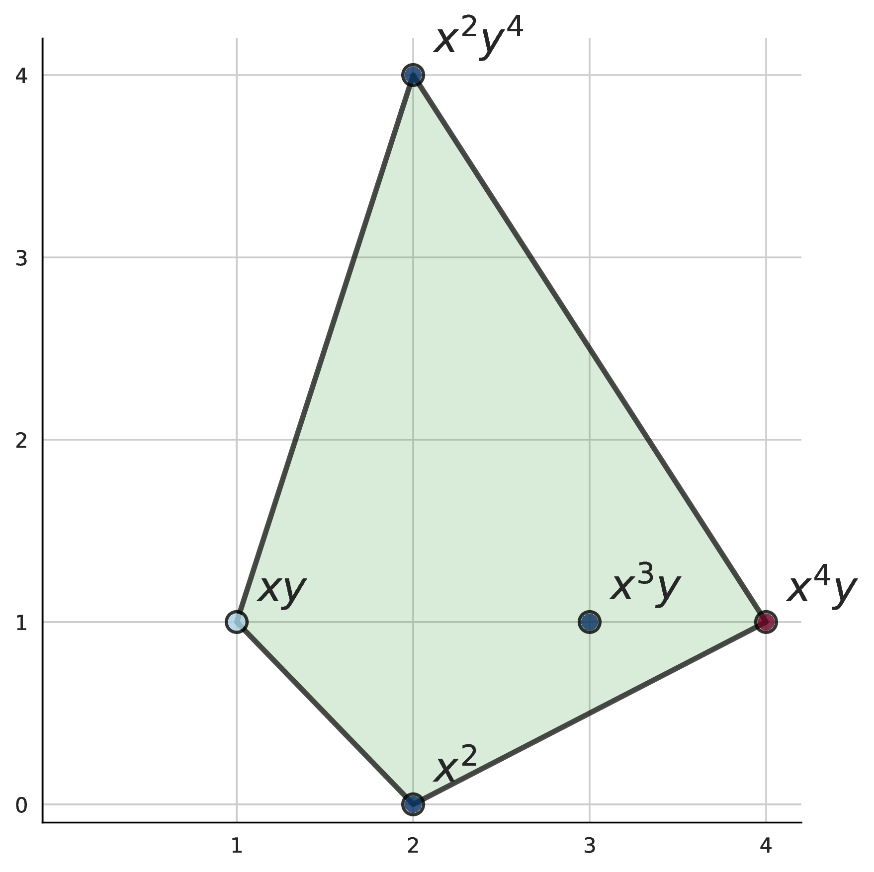
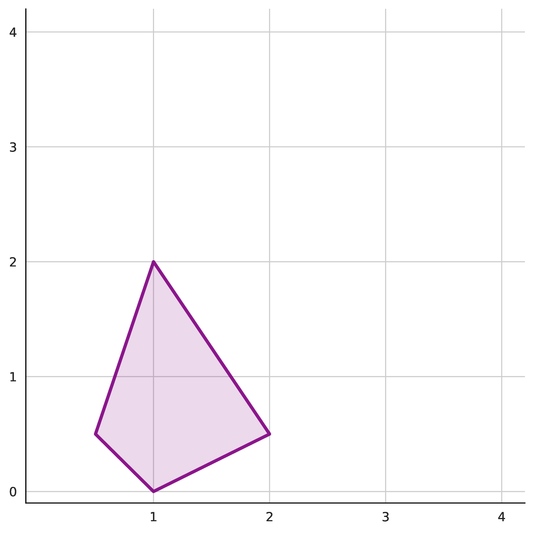
A classical result [2] constrains which monomials can appear in a valid basis: they must lie within the half Newton polytope $\frac{1}{2}N(p)$. The Newton polytope is the convex hull of a polynomial’s exponent vectors; the half Newton polytope scales this by half to define the candidate set for basis monomials. This provides an upper bound on the candidate set, but this set is still typically much larger than necessary.
Traditional methods like Newton polytope with diagonal consistency, TSSOS [4] (term sparsity), and Chordal-TSSOS [5] (chordal sparsity in the SDP) provide rule-based approaches to reducing basis size. However, they often produce bases that are still much larger than necessary in practice.
Method: Learning to Predict Compact Bases
We frame basis selection as a sequence prediction problem and train a Transformer to solve it. Given a polynomial $p(\mathbf{x})$, the model autoregressively predicts a candidate set of monomials likely to form a valid SOS basis. The predicted set is only a proposal; correctness comes from downstream SDP verification and expansion.
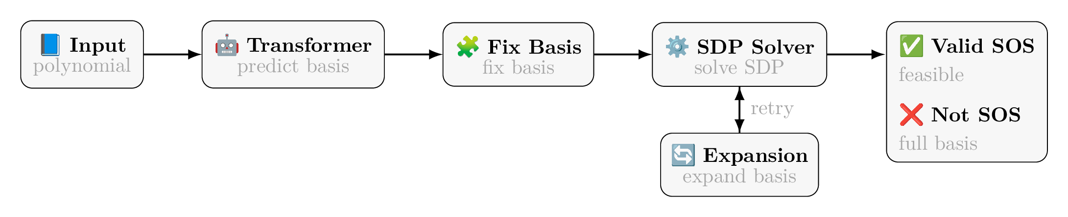
Our approach operates in three stages:
Stage 1: Transformer-Based Basis Prediction
We tokenize polynomials using a monomial-level embedding scheme from [3]. Each term is represented as a sequence of tokens encoding the coefficient and exponents. For example, the term $4x_1^4$ becomes “C4.0 E4 E0” (coefficient 4.0, $x_1$ to the 4th power, $x_2$ to the 0th power), while $12x_1^2x_2^2$ becomes “C12.0 E2 E2”. The model generates basis monomials autoregressively until producing an end-of-sequence token.
Training targets are not unique because many different bases can certify the same polynomial. To build supervised data, we use reverse sampling: sample a monomial basis $B$, draw a random PSD matrix $Q$, and compute $p(\mathbf{x}) = \mathbf{z}_B(\mathbf{x})^\top Q \, \mathbf{z}_B(\mathbf{x})$. This guarantees that each synthesized polynomial comes with at least one valid basis by construction, and these sampled bases are often close to minimal.
Stage 2: Coverage Repair
A predicted basis must satisfy a necessary condition: every monomial in the polynomial’s support must be expressible as a product of two basis monomials. For example, the set $\{x_1^2, x_1x_2, 1\}$ cannot be a basis for $p(x_1, x_2) = 4x_1^4 + 12x_1^2x_2^2 + 9x_2^4 + 1$, since none of the products of these monomials forms $x_2^4$, which appears in the support of $p$.
If the predicted basis violates this condition, we apply a greedy repair algorithm that iteratively adds monomials covering the most missing support terms. This condition is necessary but not sufficient: support coverage alone does not guarantee SDP feasibility.
Stage 3: Iterative Expansion with Verification
If the coverage-repaired basis still fails to yield a feasible SDP, we expand it systematically. Rather than adding monomials arbitrarily, we rank candidates using a permutation-based scoring mechanism:
We run the Transformer on multiple random permutations of the polynomial’s variables, then score each monomial by how frequently it appears across predictions. Monomials with higher scores are added first during expansion. If expansion is still unsuccessful, we continue enlarging the basis until we recover the standard candidate set, which matches the classical SOS pipeline.
Empirical Evaluation
Across training and evaluation, we generate and process over 200 million synthetic SOS polynomials. The results depend strongly on polynomial structure, and favorable structures yield the largest computational savings.
Large-Scale Performance
We first demonstrate performance on challenging large-scale configurations, comparing against state-of-the-art SOS solvers: SoS.jl [6] (standard Newton polytope), TSSOS [4] (term sparsity), and Chordal-TSSOS [5] (term sparsity with chordal extension).
| Configuration | Ours | SoS.jl | TSSOS | Chordal-TSSOS |
|---|---|---|---|---|
| 6 vars, deg 20 | 5.64s | 119.98s | 86.53s | 105.54s |
| 6 vars, deg 40 | 42.8s | – | – | – |
| 8 vars, deg 20 | 1.46s | 3037.85s | 2674.50s | 3452.98s |
| 100 vars, deg 10 | 18.3s | – | – | – |
Table shows average solve time in seconds. “–” indicates out-of-memory or timeout.
Our method demonstrates strong scalability advantages on structured instances. For the 8-variable, degree-20 configuration in this table, we observe over 1800x speedup relative to standard Newton-polytope-based solving. More significantly, our method successfully solves problems where all baselines fail due to memory constraints, including 6 variables at degree 40 and 100 variables at degree 10.
Results on Sparse Polynomials
We benchmark against the standard Newton polytope method across polynomials with different underlying structures. The table below shows results for polynomials that were sampled using a sparse matrix $Q$.
| Variables | Degree | Basis Size (Ours) | Basis Size (Newton) | Time (Ours) | Time (Newton) | Speedup |
|---|---|---|---|---|---|---|
| 4 | 6 | 15 | 18 | 0.23s | 0.20s | 0.9× |
| 6 | 12 | 27 | 40 | 0.57s | 1.20s | 2.1× |
| 8 | 20 | 27 | 28 | 0.62s | 15.3s | 25× |
| 6 | 20 | 73 | 233 | 7.4s | 1606s | 217× |
Comparison with the standard Newton-polytope basis on sparse SOS polynomials. Our method often finds substantially smaller bases, which leads to large reductions in SDP solve time on larger instances.
On small problems, the overhead of running a Transformer offsets any gains from reduced basis size. However, as problems scale, the difference in basis size translates to substantial savings in SDP solve time. For the 6-variable, degree-20 case, the predicted basis (73 monomials) is approximately 3× smaller than the Newton polytope basis (233 monomials), reducing solve time from 1606 seconds to 7.4 seconds.
Dependence on Polynomial Structure
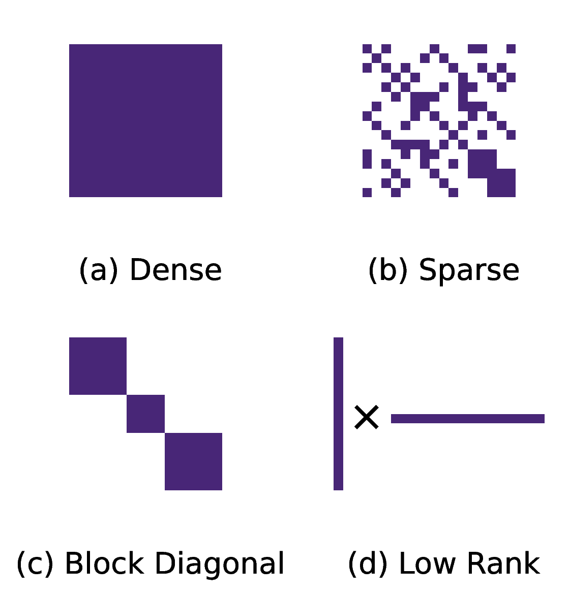
Performance is not uniform across polynomial families. Raw prediction accuracy before repair varies with underlying polynomial structure.
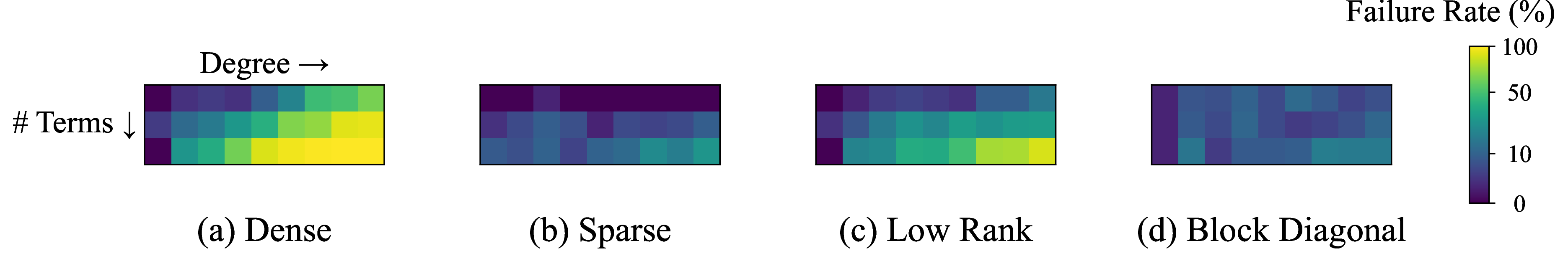
These heatmaps illustrate that polynomial structure significantly affects prediction difficulty. Sparse and block-diagonal polynomials exhibit regularities in their coefficient matrices that the Transformer learns to exploit, achieving 85–95% success rates. Dense and low-rank cases lack such structure, making the prediction task inherently harder.
This behavior is consistent with expectations: basis selection is easier when the underlying problem has exploitable structure. Notably, many practical SOS applications (control Lyapunov functions, sparse polynomial optimization) fall into the favorable categories.
Repair Mechanisms
Raw prediction accuracy alone does not determine algorithm performance. When the Transformer’s initial basis is insufficient, the repair mechanisms attempt to recover a valid basis.
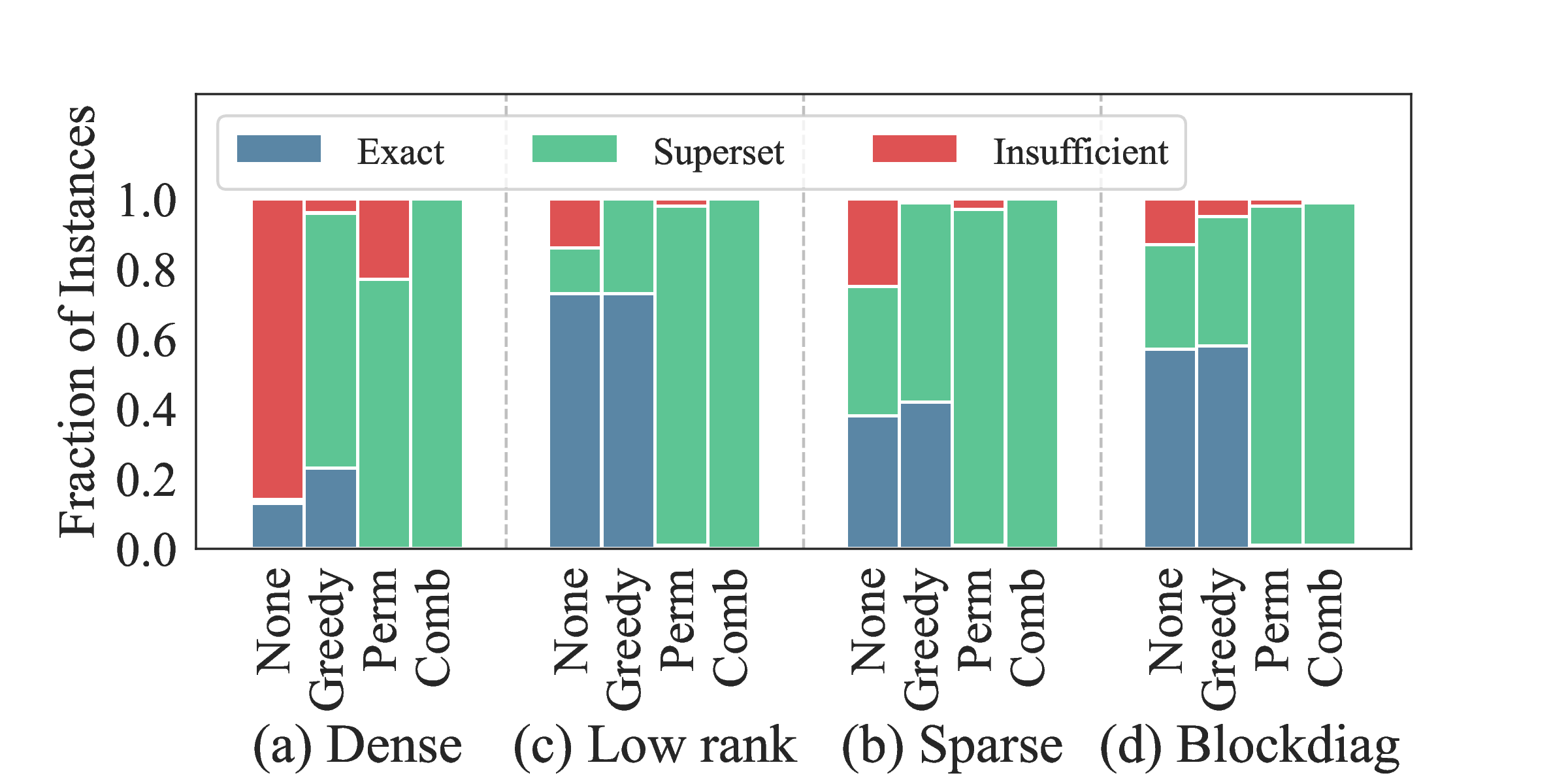
This figure summarizes post-repair outcomes. The greedy coverage repair handles most failures cheaply—it simply adds missing monomials to satisfy necessary conditions. The permutation-based expansion handles the harder cases where the SDP itself fails, using ensemble predictions to guide monomial selection.
The combined approach reduces insufficient cases to under 5% across all structures. Even when repair is needed, the final basis typically remains compact enough to preserve computational advantages over baselines.
Runtime Analysis
A relevant consideration is whether neural network inference adds substantial overhead. We analyze the runtime breakdown to understand the computational costs.
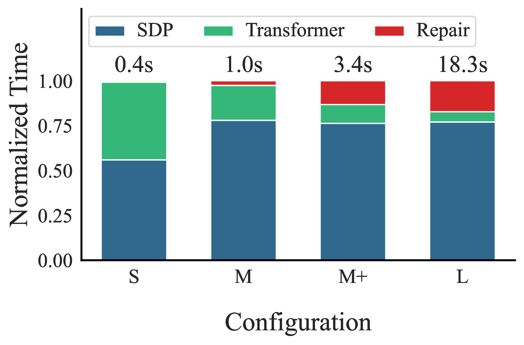
The results show that SDP solving dominates the runtime. For larger problems, the SDP accounts for 75–80% of total runtime, while Transformer inference and repair overhead are comparatively small. This supports the premise that reducing basis size is the primary factor affecting overall performance, and the cost of prediction is acceptable. In other words, even imperfect basis prediction can pay off if it shrinks the SDP enough.
Limitations
Synthetic data dependence. The evaluation relies on synthetic polynomial generation; real-world SOS benchmarks would strengthen the empirical case.
Distribution shift risk. Performance may degrade on polynomial families that differ substantially from the training distribution.
Limited gains on small instances. On small problems, model inference and repair overhead can offset basis reduction gains.
Structure-dependent benefit. The largest improvements occur on sparse and structured families; dense or weakly structured cases are harder.
No acceleration for non-SOS instances. For polynomials that are not SOS, proving non-existence still requires recovering the full Newton-polytope candidate basis. Relative to the standard Newton-polytope pipeline, the added overhead ranges from 2.2x (small problems) to 1.05x (larger ones).
Conclusion
Overall, the main idea is simple: use a Transformer to propose a small SOS basis, then rely on verification and repair to keep the pipeline correct. On structured instances, this can shrink the resulting SDP enough to produce large speedups, and in our synthetic benchmarks it enables cases that standard baselines cannot solve within memory or time limits.
More broadly, this is an example of a promising design pattern for scientific machine learning: let learned models make useful proposals, but leave final certification to exact methods.
@misc{pelleriti2025neuralsumofsquarescertifyingnonnegativity,
      title={Neural Sum-of-Squares: Certifying the Nonnegativity of Polynomials with Transformers},
      author={Nico Pelleriti and Christoph Spiegel and Shiwei Liu and David Martínez-Rubio and Max Zimmer and Sebastian Pokutta},
      year={2025},
      eprint={2510.13444},
      archivePrefix={arXiv},
      primaryClass={cs.LG},
      url={https://arxiv.org/abs/2510.13444},
}
References
[1] Parrilo, P. A. (2003). Semidefinite programming relaxations for semialgebraic problems. Mathematical Programming, 96(2), 293–320.
[2] Reznick, B. (1978). Extremal PSD forms with few terms. Duke Mathematical Journal, 45(2), 363–374.
[3] Kera, H., Pelleriti, N., Ishihara, Y., Zimmer, M., & Pokutta, S. (2025). Computational Algebra with Attention: Transformer Oracles for Border Basis Algorithms. arXiv preprint arXiv:2505.23696.
[4] Wang, J., Magron, V., & Lasserre, J. B. (2019). TSSOS: A Moment-SOS Hierarchy That Exploits Term Sparsity. SIAM Journal on Optimization, 31, 30–58.
[5] Wang, J., Magron, V., & Lasserre, J. B. (2020). Chordal-TSSOS: A Moment-SOS Hierarchy That Exploits Term Sparsity with Chordal Extension. SIAM Journal on Optimization, 31, 114–141.
[6] Weisser, T., Legat, B., Coey, C., Kapelevich, L., & Vielma, J. P. (2019). Polynomial and Moment Optimization in Julia and JuMP. JuliaCon 2019.