<?xml version="1.0" encoding="utf-8"?><feed xmlns="http://www.w3.org/2005/Atom" ><generator uri="https://jekyllrb.com/" version="3.10.0">Jekyll</generator><link href="https://www.pelleriti.org/feed.xml" rel="self" type="application/atom+xml" /><link href="https://www.pelleriti.org/" rel="alternate" type="text/html" /><updated>2026-03-03T09:54:26+00:00</updated><id>https://www.pelleriti.org/feed.xml</id><title type="html">Home</title><subtitle>PhD in Mathematics at TU Berlin. Building interactive agentic systems for mathematical and scientific discovery.</subtitle><author><name>Nico Pelleriti</name><email>pelleriti@zib.de</email></author><entry><title type="html">Computational Algebra with Attention: Transformer Oracles for Border Basis Algorithms</title><link href="https://www.pelleriti.org/posts/2025/12/computational-algebra-with-attention/" rel="alternate" type="text/html" title="Computational Algebra with Attention: Transformer Oracles for Border Basis Algorithms" /><published>2025-12-01T00:00:00+00:00</published><updated>2025-12-01T00:00:00+00:00</updated><id>https://www.pelleriti.org/posts/2025/12/borderbasis</id><content type="html" xml:base="https://www.pelleriti.org/posts/2025/12/computational-algebra-with-attention/"><![CDATA[<p><em>This post accompanies our paper accepted at <strong>NeurIPS 2025</strong>: <a href="https://arxiv.org/abs/2505.23696">Computational Algebra with Attention: Transformer Oracles for Border Basis Algorithms</a></em></p>

<p>Many problems in cryptography, robotics, and optimization reduce to solving polynomial equations. Gaussian elimination handles linear systems in $O(n^3)$, but polynomial systems are another story: complexity explodes with degree, and classical algorithms burn most of their runtime on calculations that end up contributing nothing. We introduce the <strong>Oracle Border Basis Algorithm (OBBA)</strong>, which uses a Transformer to predict which computations actually matter—achieving speedups of up to 3.5× while guaranteeing correctness through verified fallback.</p>

<hr />

<h2 id="polynomial-system-solving-and-its-challenges">Polynomial System Solving and Its Challenges</h2>

<p>A polynomial system is a collection of equations like
$x^2 + y^2 = 1$ and $xy = 0.5$ in several variables. The goal is to
describe all common solutions. For linear systems, Gaussian elimination
does this efficiently and with very little wasted work. For polynomial
systems, the analogous algorithms are far more expensive: the number of
candidate terms and intermediate polynomials grows exponentially, and most
of them turn out to be redundant in hindsight.</p>

<p>Our work focuses on this redundancy. We ask whether it is possible to
predict, before doing any heavy algebra, which computations are likely
to be useful—and then use those predictions to steer a classical
algorithm without sacrificing correctness.</p>

<h2 id="background-from-gaussian-elimination-to-border-bases">Background: From Gaussian Elimination to Border Bases</h2>

<p>To provide intuition, recall that Gaussian elimination offers a systematic route to <strong>row echelon form</strong> in linear algebra, simplifying linear systems to a point where solutions become directly accessible. The Border Basis Algorithm (BBA) [1] pursues an analogous goal in the polynomial setting, producing a <strong>border basis</strong>—a structured, canonical representation that encodes all solutions to a polynomial system.</p>

<p>A border basis plays a role in polynomial algebra reminiscent of row echelon form in linear algebra. Just as each row in echelon form has a distinct pivot variable, each polynomial in a border basis has a distinct leading monomial such as $x^2$. Together, these polynomials generate an <em>ideal</em>—the algebraic structure encoding all solutions to the original system.</p>

<p>Crucially, both structures are <strong>verifiable</strong>: given a candidate output, one can check whether it is valid without re-running the algorithm. This property is what enables our <em>correctness guarantee</em>.</p>

<p>One important constraint is that the BBA only applies to systems with <em>finitely many solutions</em>, analogous to requiring a linear system to have full rank. For instance, the system $x^2 + y^2 = 1$ and $x = y$ has exactly two solutions, whereas $x^2 + y^2 = 1$ alone has infinitely many (the unit circle) and falls outside the algorithm’s scope.</p>

<h2 id="the-border-basis-algorithm">The Border Basis Algorithm</h2>

<p>The core operation of the BBA mirrors Gaussian elimination: maintain a set of basis polynomials and systematically extend it by combining polynomials to eliminate terms. However, unlike linear systems, polynomial systems require working <strong>degree by degree</strong>—starting with low-degree polynomials, then progressively considering higher degrees until the basis <em>stabilizes</em>.</p>

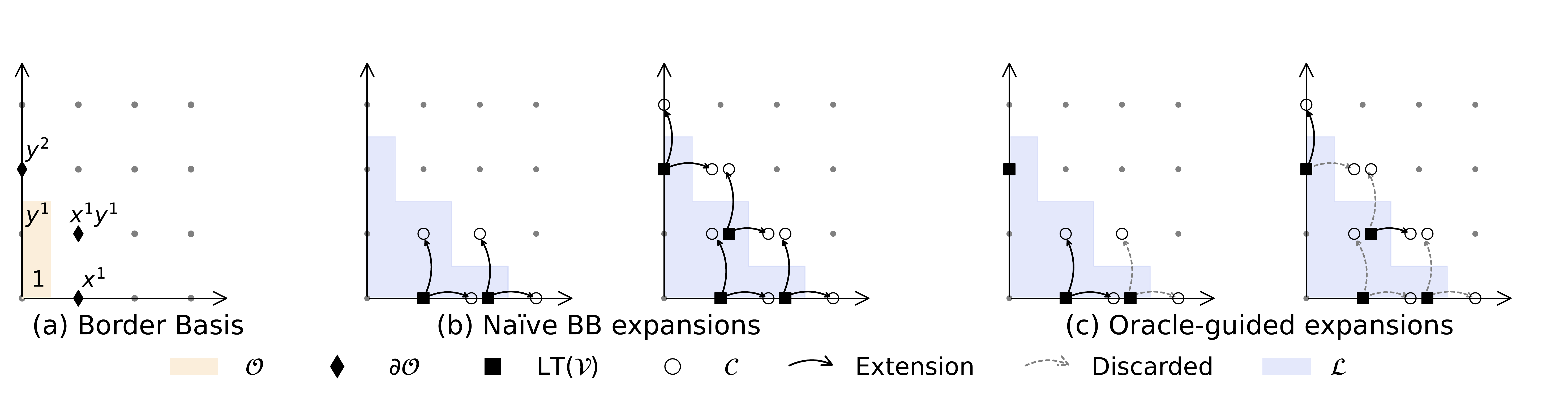
<p>Since the algorithm operates degree by degree, at any given iteration we only consider polynomials up to some maximum degree $d$. This defines the current <strong>computational universe</strong> $\mathcal{L}$—the set of all monomials up to degree $d$. For example, with two variables $x$ and $y$ at degree 2, the universe is $\mathcal{L} = \{1, x, y, x^2, xy, y^2\}$. The algorithm maintains a <strong>generator set</strong> $\mathcal{V}$ of polynomials with distinct leading terms, tracking only polynomials that lie entirely within $\mathcal{L}$; terms outside this set are deferred to later iterations.</p>

<figure class="fig-white-bg">
  <img src="/images/blogpost_figures/BorderBasisAlgo-1.png" alt="Border Basis Algorithm Visualization" />
  <figcaption>Border basis concepts: (a) A border basis with border terms \(\{y^2,xy,x\}\). (b) BBA's iterative expansion of \(\mathcal{V}\), showing leading terms: two initial polynomials yield four expansions, then eight more - though only two out of twelve were necessary. (c) The oracle approach achieves the same result with just four targeted expansions.</figcaption>
</figure>

<p>At each iteration, the algorithm proceeds as follows:</p>

<ol>
  <li><strong>Expansion</strong>: Multiply every polynomial in the current basis by every variable, creating a pool of candidate polynomials $\mathcal{V}^+$.</li>
  <li><strong>Reduction</strong>: Apply Gaussian elimination to compute a basis for the span of all candidates.</li>
  <li><strong>Filtering</strong>: Retain only those polynomials whose terms lie entirely within the computational universe $\mathcal{L}$.</li>
</ol>

<p>A candidate polynomial <strong>extends the basis</strong> if, after reduction, it produces a non-zero polynomial that was not already expressible as a combination of existing basis elements. If it reduces to zero, it was redundant—merely a consequence of polynomials already present.</p>

<p>On the other hand, we call $\mathcal{V}$ an $\mathcal{L}$-stable span, if after the filtering, no polynomial is retained.</p>

<h3 id="a-worked-example">A Worked Example</h3>

<p>Consider one iteration at degree 2, where the computational universe is:</p>

\[\mathcal{L} = \{1, x, y, x^2, xy, y^2\}\]

<p>and the current generator set contains two polynomials:</p>

\[\mathcal{V} = \{x - 1,\; x^2 + y^2 - 1\}\]

<p><strong>Step 1: Expansion.</strong> Multiply each polynomial in $\mathcal{V}$ by each variable ($x$ and $y$) to form $\mathcal{V}^+$:</p>

<table>
  <thead>
    <tr>
      <th style="text-align: center">Expansion</th>
      <th style="text-align: center">Result</th>
    </tr>
  </thead>
  <tbody>
    <tr>
      <td style="text-align: center">$x \cdot (x - 1)$</td>
      <td style="text-align: center">$x^2 - x$</td>
    </tr>
    <tr>
      <td style="text-align: center">$y \cdot (x - 1)$</td>
      <td style="text-align: center">$xy - y$</td>
    </tr>
    <tr>
      <td style="text-align: center">$x \cdot (x^2 + y^2 - 1)$</td>
      <td style="text-align: center">$x^3 + xy^2 - x$</td>
    </tr>
    <tr>
      <td style="text-align: center">$y \cdot (x^2 + y^2 - 1)$</td>
      <td style="text-align: center">$x^2y + y^3 - y$</td>
    </tr>
  </tbody>
</table>

<p><strong>Step 2: Reduction.</strong> Apply Gaussian elimination to compute a basis for the span of $\mathcal{V}^+$:</p>

<ul>
  <li>$x^2 - x$ reduces (using $x^2 + y^2 - 1$) to $y^2 + x - 1$</li>
  <li>$xy - y$ cannot be further reduced</li>
</ul>

<p><strong>Step 3: Filtering.</strong> Retain only polynomials whose terms lie entirely within $\mathcal{L}$. The last two expansions contain $x^3$, $xy^2$, $x^2y$, and $y^3$—monomials outside the computational universe—and are therefore discarded. This yields two new polynomials that extend $\mathcal{V}$:</p>

\[\mathcal{V} \leftarrow \{x - 1,\; x^2 + y^2 - 1,\; y^2 + x - 1,\; xy - y\}\]

<p>Of 4 candidates, only 2 were useful; the remaining 2 fell outside the current scope. This was a minimal example—as problems grow, the ratio of redundant to useful reductions becomes substantially worse. In Gaussian elimination, redundant rows reduce to zero; in border basis computation, the <em>majority</em> of generated candidates reduce to zero.</p>

<h3 id="computational-redundancy-in-the-border-basis-algorithm">Computational Redundancy in the Border Basis algorithm</h3>

<p>A linear system can be overdetermined: some equations are linear combinations of others. 
In Gaussian elimination, this appears as rows that reduce to zero—redundant equations that, if identified in advance, could simply be omitted.</p>

<p>The Border Basis Algorithm suffers from the same redundancy at a far worse ratio. The space of candidate expansions grows combinatorially, yet the survivors—polynomials that remain nonzero after reduction—are sparse. We pay the full cost of generating and reducing every candidate, only to learn that most were unnecessary.</p>

<p>This is precisely the inefficiency our Transformer oracle addresses.</p>

<h2 id="a-neural-oracle-for-expansion-selection">A Neural Oracle for Expansion Selection</h2>

<p>Rather than exhaustively expanding all candidates and discovering afterward that most reduce to zero, we predict in advance which expansions are likely to extend the basis. We train a Transformer that takes the current polynomial set $\mathcal{V}$ and monomial universe $\mathcal{L}$ as input, and outputs a subset $\mathcal{C} \subseteq \mathcal{V}^+$ of expansions predicted to survive reduction and filtering.</p>

<p>The Border Basis Algorithm operates degree-by-degree, so each iteration provides a natural training example: given $\mathcal{V}$ and $\mathcal{L}$, we record which expansions survived. Running the algorithm once yields a full dataset of minimal expansions.</p>

<p>Of course, a neural network can miss crucial expansions. But border bases are far easier to verify than to compute—so we check the result and fall back to the standard algorithm if needed. This gives us the best of both worlds:</p>

<ul>
  <li>Accurate predictions → maximum speedup</li>
  <li>False positives → additional overhead from extra reductions</li>
  <li>False negatives → verification fails, fallback to full expansion</li>
</ul>

<h2 id="tokenizing-polynomials">Tokenizing Polynomials</h2>

<p>Polynomials can contain thousands of terms. A naive tokenization—one token per coefficient, one per exponent, plus operators—blows up quickly. Even $x + 2$ becomes seven tokens:</p>

<div class="language-plaintext highlighter-rouge"><div class="highlight"><pre class="highlight"><code>C1, E1, E0, +, C2, E0, E0
</code></pre></div></div>

<p>With $n$ variables, each term costs $(n+1)$ tokens. This is prohibitive.</p>

<p>We encode each term as a single token. Instead of breaking $3x^2y$ into separate tokens for the coefficient and each exponent, we combine everything into one embedding:</p>

\[\text{embed}(\text{term}) = \text{embed}_{\text{coef}}(c) + \frac{1}{n} \sum_{i=1}^n \text{embed}_{\text{var}_i}(a_i) + \text{embed}_{\text{sep}}\]

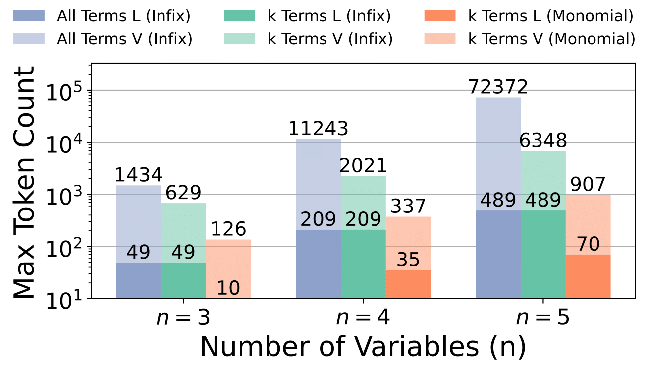
<p>This matches how polynomial algebra actually works: operations combine terms with matching monomial structure. With one token per term, attention can directly compare terms across polynomials instead of first figuring out which token clusters belong together.</p>

<figure class="fig-white-bg fig-75">
  <img src="/images/blogpost_figures/token_count.png" alt="Token Efficiency" />
  <figcaption>Term-level embedding plus truncation dramatically reduce input size.</figcaption>
</figure>

<p>We also truncate to the first $k$ leading terms of each polynomial—these typically determine which expansions survive. Together, these choices drastically cut token count and let us handle much larger systems.</p>

<h2 id="generating-training-data">Generating Training Data</h2>

<p>The BBA only applies to systems with finitely many solutions. Random polynomials almost never have this property—they have either no solutions or infinitely many.</p>

<p>We sample in reverse: start with a valid border basis (which by definition has finitely many solutions), then apply random transformations to generate diverse examples while preserving the algebraic structure.</p>

<h2 id="experimental-results">Experimental Results</h2>

<p>We evaluate on randomly generated polynomial systems over finite fields—a setting common in cryptographic applications and algebraic coding theory. Each system has a known, finite solution set, enabling automatic verification of correctness.</p>

<figure class="fig-white-bg">
  <img src="/images/blogpost_figures/runtime_barplots-1.png" alt="Runtime Results" />
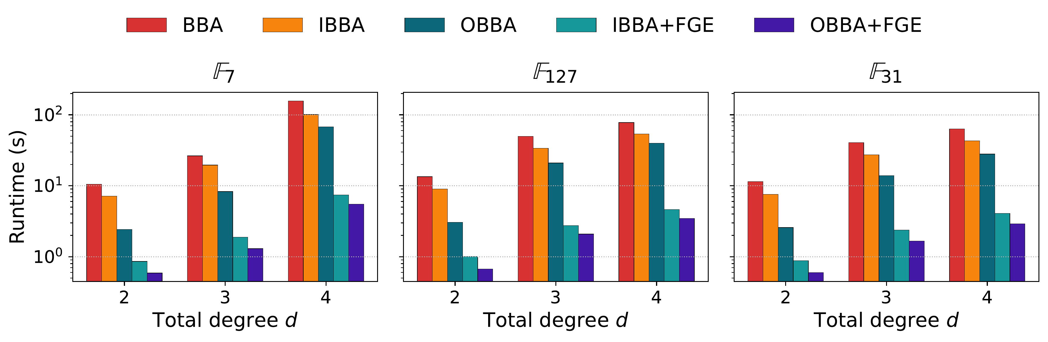
  <figcaption>Runtime comparison (log scale) across different problem configurations. OBBA consistently outperforms the baseline BBA, with speedups increasing for more challenging problems.</figcaption>
</figure>

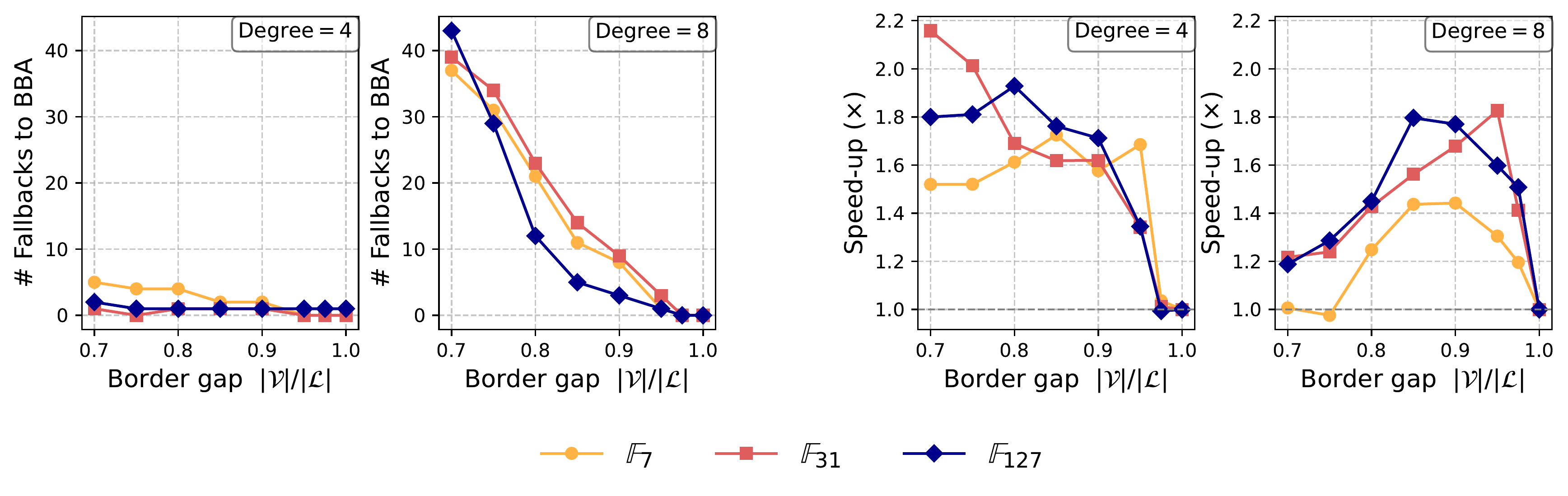
<p>Crucially, the oracle generalizes well beyond its training distribution. Models trained exclusively on degree-2 polynomials successfully accelerate degree-3 and degree-4 problems—instances 10–100× harder than anything seen during training. This means we can generate training data cheaply by solving easy problems, then deploy the trained model on problems that are significantly harder.</p>

<figure class="fig-white-bg">
  <img src="/images/blogpost_figures/ood_speedup-1.png" alt="Out-of-Distribution Performance" />
  <figcaption>
    Speedup as problem difficulty increases for systems with 4 variables. OBBA still achieves strong speedups even when solving problems harder than those it was trained on (higher-degree polynomials). The ratio $\frac{|\mathcal{V}|}{|\mathcal{L}|}$ helps us decide how often to use the oracle: if this ratio is close to $1$, we are nearly done, but if it is much smaller, more steps are needed.
  </figcaption>
</figure>

<h3 id="numerical-results">Numerical Results</h3>

<p>For 5-variable polynomial systems over $\mathbb{F}_{31}$ (a prime field commonly used in computational algebra):</p>

<table>
  <thead>
    <tr>
      <th style="text-align: center">Degree</th>
      <th style="text-align: center">Baseline BBA</th>
      <th style="text-align: center">Our Method</th>
      <th style="text-align: center">Speedup</th>
    </tr>
  </thead>
  <tbody>
    <tr>
      <td style="text-align: center">2 (in-distribution)</td>
      <td style="text-align: center">11.4s</td>
      <td style="text-align: center">0.60s</td>
      <td style="text-align: center">19×</td>
    </tr>
    <tr>
      <td style="text-align: center">3 (out-of-distribution)</td>
      <td style="text-align: center">40.7s</td>
      <td style="text-align: center">1.7s</td>
      <td style="text-align: center">24×</td>
    </tr>
    <tr>
      <td style="text-align: center">4 (out-of-distribution)</td>
      <td style="text-align: center">136.7s</td>
      <td style="text-align: center">5.6s</td>
      <td style="text-align: center">24×</td>
    </tr>
  </tbody>
</table>

<p>The out-of-distribution results are notable: problems significantly harder than anything in training, yet the oracle still achieves greater than 20× speedup. When the oracle does make prediction errors, the verification step detects them and triggers fallback—correctness is never compromised.</p>

<h2 id="whats-missing">What’s Missing</h2>

<p>We only go up to 5 variables over finite fields. Scaling further will likely need larger models and different training techniques. While out-of-distribution generalization is strong, it has limits—push too far from the training distribution and the oracle starts missing expansions. The algorithm stays correct (fallback kicks in), but speedups shrink.</p>

<h2 id="looking-ahead">Looking Ahead</h2>

<p>Polynomial systems can encode many of the hardest problems in computation: classic NP-hard problems such as MAX-CUT can be written as polynomial optimization tasks. At the same time, polynomial constraints are often far more expressive than linear ones—some feasible sets that require exponentially many linear inequalities admit succinct descriptions with only a few polynomial equations. By designing a tokenizer that exploits this algebraic structure, we obtain highly compressed representations that fit within Transformer-scale context windows.</p>

<p>This approach extends in principle to <strong>polynomial optimization</strong> and <strong>numerical root-finding</strong>—tools that play central roles in robotics, computer vision, and combinatorial optimization. The general pattern is to use learned predictions to guide and prune a classical algorithm’s search, while retaining a fast verification step so that any accepted solution comes with a clear correctness certificate. Border bases are a clean first testbed. The more interesting story is broader: wherever a hard problem has a compact algebraic encoding and a fast verifier, there’s an opportunity to drop in a learned oracle.</p>

<hr />

<p><strong>Paper:</strong> <a href="https://arxiv.org/abs/2505.23696">Computational Algebra with Attention: Transformer Oracles for Border Basis Algorithms</a> (NeurIPS 2025)</p>

<p><strong>Code:</strong> <a href="https://github.com/HiroshiKERA/OracleBorderBasis">github.com/HiroshiKERA/OracleBorderBasis</a></p>

<div class="language-bibtex highlighter-rouge"><div class="highlight"><pre class="highlight"><code><span class="nc">@inproceedings</span><span class="p">{</span><span class="nl">kera2025computational</span><span class="p">,</span>
      <span class="na">title</span><span class="p">=</span><span class="s">{Computational Algebra with Attention: Transformer Oracles for Border Basis Algorithms}</span><span class="p">,</span> 
      <span class="na">author</span><span class="p">=</span><span class="s">{Hiroshi Kera and Nico Pelleriti and Yuki Ishihara and Max Zimmer and Sebastian Pokutta}</span><span class="p">,</span>
      <span class="na">year</span><span class="p">=</span><span class="s">{2025}</span><span class="p">,</span>
      <span class="na">booktitle</span><span class="p">=</span><span class="s">{Advances in Neural Information Processing Systems (NeurIPS)}</span><span class="p">,</span>
      <span class="na">eprint</span><span class="p">=</span><span class="s">{2505.23696}</span><span class="p">,</span>
      <span class="na">archivePrefix</span><span class="p">=</span><span class="s">{arXiv}</span><span class="p">,</span>
      <span class="na">primaryClass</span><span class="p">=</span><span class="s">{cs.LG}</span><span class="p">,</span>
      <span class="na">url</span><span class="p">=</span><span class="s">{https://arxiv.org/abs/2505.23696}</span><span class="p">,</span> 
<span class="p">}</span>
</code></pre></div></div>

<h2 id="references">References</h2>

<p>[1] Kehrein and Kreuzer. Computing border bases. <em>Journal of Pure and Applied Algebra</em>, 205(2):279–295, 2006.</p>]]></content><author><name>Nico Pelleriti</name><email>pelleriti@zib.de</email></author><category term="Transformer" /><category term="Computational Algebra" /><category term="Border Basis" /><summary type="html"><![CDATA[This post accompanies our paper accepted at NeurIPS 2025: Computational Algebra with Attention: Transformer Oracles for Border Basis Algorithms]]></summary></entry><entry><title type="html">Neural Sum-of-Squares: Certifying Polynomial Nonnegativity with Transformers</title><link href="https://www.pelleriti.org/posts/2025/12/neural-sum-of-squares/" rel="alternate" type="text/html" title="Neural Sum-of-Squares: Certifying Polynomial Nonnegativity with Transformers" /><published>2025-12-01T00:00:00+00:00</published><updated>2025-12-01T00:00:00+00:00</updated><id>https://www.pelleriti.org/posts/2025/12/sos</id><content type="html" xml:base="https://www.pelleriti.org/posts/2025/12/neural-sum-of-squares/"><![CDATA[<p><em>This post accompanies our ICLR 2026 paper: <a href="https://arxiv.org/abs/2510.13444">Neural Sum-of-Squares: Certifying the Nonnegativity of Polynomials with Transformers</a></em></p>

<p>Many problems in control, robotics, and optimization reduce to proving that a polynomial is globally nonnegative.
A standard approach is to search for a <em>Sum-of-Squares (SOS)</em> decomposition, which turns the task into a <em>Semidefinite Program (SDP)</em>.
The bottleneck is scale: SDP size grows rapidly with polynomial degree and variable count, so even moderately sized instances can become impractical.</p>

<p>In this work, we develop a learning-augmented SOS pipeline that uses a Transformer to predict a much smaller monomial basis for the certificate search.
The model does not certify nonnegativity by itself; it proposes a smaller search space for the downstream SDP.
We still verify every candidate with an SDP solver, and if a candidate is insufficient we repair and expand it until we recover a valid certificate or fall back to the standard candidate set.</p>

<hr />

<h2 id="the-nonnegativity-certification-problem">The Nonnegativity Certification Problem</h2>

<p>A central subproblem in polynomial optimization is certifying that a fixed polynomial is globally nonnegative. This subproblem arises, for instance, when searching for the largest $\lambda$ such that $p(x)-\lambda$ remains nonnegative; in this post, we focus only on the certification step.</p>

<p>For illustration, consider the simple example:</p>

\[p(x_1, x_2) = 4x_1^4 + 12x_1^2x_2^2 + 9x_2^4 + 1\]

<p>Is this polynomial always nonnegative? One way to verify this is to write it as a <strong>Sum-of-Squares (SOS)</strong>:</p>

\[p(x_1, x_2) = (2x_1^2 + 3x_2^2)^2 + 1^2\]

<p>Since any sum of squares is clearly nonnegative, an <em>SOS decomposition</em> serves as a certificate of nonnegativity. The key insight from <a href="#ref-1">[1]</a> is that checking whether such a decomposition exists can be formulated as a <em>Semidefinite Program</em>.</p>

<h2 id="from-sos-to-semidefinite-programming">From SOS to Semidefinite Programming</h2>

<p>A polynomial $p(\mathbf{x})$ is SOS if and only if there exists a positive semidefinite matrix $Q$ such that:</p>

\[p(\mathbf{x}) = \mathbf{z}(\mathbf{x})^\top Q \, \mathbf{z}(\mathbf{x})\]

<p>where $\mathbf{z}(\mathbf{x})$ is a vector of monomials (the <em>basis</em>). For our example, the hand-written decomposition $(2x_1^2 + 3x_2^2)^2 + 1^2$ corresponds to choosing $\mathbf{z}(\mathbf{x}) = [1, x_1^2, x_2^2]^\top$, where expanding the quadratic form yields the original polynomial.</p>

<p>Choosing $\mathbf{z}(\mathbf{x})$ is the key design choice: a larger basis makes the SDP easier to formulate but often much more expensive to solve.
For a degree-$2d$ polynomial, any SOS representation uses squared polynomials of degree at most $d$, so the standard basis contains all monomials of degree at most $d$.
For this degree-4 example, that gives:</p>

\[\mathbf{z}(\mathbf{x}) = [1, x_1, x_2, x_1x_2, x_1^2, x_2^2]^\top\]

<p>This gives a 6×6 matrix $Q$ to optimize over. However, the same SOS decomposition can be computed using a much smaller basis:</p>

\[\mathbf{z}'(\mathbf{x}) = [1, x_1^2, x_2^2]^\top\]

<p>with the 3×3 matrix:</p>

\[Q = \begin{pmatrix} 1 &amp; 0 &amp; 0 \\ 0 &amp; 4 &amp; 6 \\ 0 &amp; 6 &amp; 9 \end{pmatrix}\]

<p>The computational cost of solving an SDP scales polynomially in the matrix dimension—so using a basis of size 3 instead of 6 yields substantial savings. 
For larger problems with dozens of variables and high degrees, the size of the basis often determines if the problem is tractable at all.</p>

<h2 id="the-basis-selection-bottleneck">The Basis Selection Bottleneck</h2>

<p>A central computational challenge in SOS programming is <strong>basis selection</strong>: finding a compact set of monomials that admits an SOS decomposition while keeping the SDP as small as possible.</p>

<figure class="fig-side-by-side fig-white-bg" style="max-width: 80%;">
  <div class="subfig">
    <div class="sublabel">(a)</div>
    <img src="/images/blogpost_figures/newton_polytope-1.png" alt="Newton Polytope" />
  </div>
  <div class="subfig">
    <div class="sublabel">(b)</div>
    <img src="/images/blogpost_figures/half_newton_polytope-1.png" alt="Half Newton Polytope" />
  </div>
  <figcaption>(a) The Newton polytope of a polynomial captures geometric constraints on which monomials can appear in an SOS basis. (b) The half Newton polytope defines the candidate set for basis monomials.</figcaption>
</figure>

<p>A classical result <a href="#ref-2">[2]</a> constrains which monomials can appear in a valid basis: they must lie within the <em>half Newton polytope</em> $\frac{1}{2}N(p)$. The Newton polytope is the convex hull of a polynomial’s exponent vectors; the half Newton polytope scales this by half to define the candidate set for basis monomials. This provides an upper bound on the candidate set, but this set is still typically much larger than necessary.</p>

<p>Traditional methods like Newton polytope with diagonal consistency, TSSOS <a href="#ref-4">[4]</a> (term sparsity), and Chordal-TSSOS <a href="#ref-5">[5]</a> (chordal sparsity in the SDP) provide rule-based approaches to reducing basis size.
However, they often produce bases that are still much larger than necessary in practice.</p>

<h2 id="method-learning-to-predict-compact-bases">Method: Learning to Predict Compact Bases</h2>

<p>We frame basis selection as a sequence prediction problem and train a Transformer to solve it.
Given a polynomial $p(\mathbf{x})$, the model autoregressively predicts a candidate set of monomials likely to form a valid SOS basis.
The predicted set is only a proposal; correctness comes from downstream SDP verification and expansion.</p>

<figure class="fig-white-bg">
  <img src="/images/blogpost_figures/schematic_large-1.png" alt="Schematic Overview" />
  <figcaption>Overview of our learning-augmented SOS framework: (i) A Transformer predicts a compact basis from the polynomial, (ii) the basis is adjusted to satisfy necessary conditions, and (iii) an SDP is solved with iterative expansion if needed.</figcaption>
</figure>

<p>Our approach operates in three stages:</p>

<h3 id="stage-1-transformer-based-basis-prediction">Stage 1: Transformer-Based Basis Prediction</h3>

<p>We tokenize polynomials using a monomial-level embedding scheme from <a href="#ref-3">[3]</a>. Each term is represented as a sequence of tokens encoding the coefficient and exponents. For example, the term $4x_1^4$ becomes “C4.0 E4 E0” (coefficient 4.0, $x_1$ to the 4th power, $x_2$ to the 0th power), while $12x_1^2x_2^2$ becomes “C12.0 E2 E2”. The model generates basis monomials autoregressively until producing an end-of-sequence token.</p>

<p>Training targets are not unique because many different bases can certify the same polynomial.
To build supervised data, we use <strong>reverse sampling</strong>: sample a monomial basis $B$, draw a random PSD matrix $Q$, and compute $p(\mathbf{x}) = \mathbf{z}_B(\mathbf{x})^\top Q \, \mathbf{z}_B(\mathbf{x})$.
This guarantees that each synthesized polynomial comes with at least one valid basis by construction, and these sampled bases are often close to minimal.</p>

<figure class="fig-50 fig-white-bg">
  <img src="/images/blogpost_figures/matrix_structures-1.png" alt="Matrix Structures" />
  <figcaption>We train on diverse polynomial families generated from different PSD matrix structures: dense full-rank, sparse, block diagonal, and low-rank.</figcaption>
</figure>

<h3 id="stage-2-coverage-repair">Stage 2: Coverage Repair</h3>

<p>A predicted basis must satisfy a necessary condition: every monomial in the polynomial’s support must be expressible as a product of two basis monomials. For example, the set $\{x_1^2, x_1x_2, 1\}$ cannot be a basis for $p(x_1, x_2) = 4x_1^4 + 12x_1^2x_2^2 + 9x_2^4 + 1$, since none of the products of these monomials forms $x_2^4$, which appears in the support of $p$.</p>

<p>If the predicted basis violates this condition, we apply a greedy repair algorithm that iteratively adds monomials covering the most missing support terms.
This condition is necessary but not sufficient: support coverage alone does not guarantee SDP feasibility.</p>

<h3 id="stage-3-iterative-expansion-with-verification">Stage 3: Iterative Expansion with Verification</h3>

<p>If the coverage-repaired basis still fails to yield a feasible SDP, we expand it systematically. Rather than adding monomials arbitrarily, we rank candidates using a <strong>permutation-based scoring</strong> mechanism:</p>

<p>We run the Transformer on multiple random permutations of the polynomial’s variables, then score each monomial by how frequently it appears across predictions. Monomials with higher scores are added first during expansion.
If expansion is still unsuccessful, we continue enlarging the basis until we recover the standard candidate set, which matches the classical SOS pipeline.</p>

<h2 id="empirical-evaluation">Empirical Evaluation</h2>

<p>Across training and evaluation, we generate and process over 200 million synthetic SOS polynomials.
The results depend strongly on polynomial structure, and favorable structures yield the largest computational savings.</p>

<h3 id="large-scale-performance">Large-Scale Performance</h3>

<p>We first demonstrate performance on challenging large-scale configurations, comparing against state-of-the-art SOS solvers: SoS.jl <a href="#ref-6">[6]</a> (standard Newton polytope), TSSOS <a href="#ref-4">[4]</a> (term sparsity), and Chordal-TSSOS <a href="#ref-5">[5]</a> (term sparsity with chordal extension).</p>

<table>
  <thead>
    <tr>
      <th style="text-align: left">Configuration</th>
      <th style="text-align: center">Ours</th>
      <th style="text-align: center">SoS.jl</th>
      <th style="text-align: center">TSSOS</th>
      <th style="text-align: center">Chordal-TSSOS</th>
    </tr>
  </thead>
  <tbody>
    <tr>
      <td style="text-align: left">6 vars, deg 20</td>
      <td style="text-align: center">5.64s</td>
      <td style="text-align: center">119.98s</td>
      <td style="text-align: center">86.53s</td>
      <td style="text-align: center">105.54s</td>
    </tr>
    <tr>
      <td style="text-align: left">6 vars, deg 40</td>
      <td style="text-align: center">42.8s</td>
      <td style="text-align: center">–</td>
      <td style="text-align: center">–</td>
      <td style="text-align: center">–</td>
    </tr>
    <tr>
      <td style="text-align: left">8 vars, deg 20</td>
      <td style="text-align: center">1.46s</td>
      <td style="text-align: center">3037.85s</td>
      <td style="text-align: center">2674.50s</td>
      <td style="text-align: center">3452.98s</td>
    </tr>
    <tr>
      <td style="text-align: left">100 vars, deg 10</td>
      <td style="text-align: center">18.3s</td>
      <td style="text-align: center">–</td>
      <td style="text-align: center">–</td>
      <td style="text-align: center">–</td>
    </tr>
  </tbody>
</table>

<p><em>Table shows average solve time in seconds. “–” indicates out-of-memory or timeout.</em></p>

<p>Our method demonstrates strong scalability advantages on structured instances.
For the 8-variable, degree-20 configuration in this table, we observe over 1800x speedup relative to standard Newton-polytope-based solving.
More significantly, our method successfully solves problems where all baselines fail due to memory constraints, including 6 variables at degree 40 and 100 variables at degree 10.</p>

<h3 id="results-on-sparse-polynomials">Results on Sparse Polynomials</h3>

<p>We benchmark against the standard Newton polytope method across polynomials with different underlying structures. The table below shows results for polynomials that were sampled using a sparse matrix $Q$.</p>

<table>
  <thead>
    <tr>
      <th style="text-align: center">Variables</th>
      <th style="text-align: center">Degree</th>
      <th style="text-align: center">Basis Size (Ours)</th>
      <th style="text-align: center">Basis Size (Newton)</th>
      <th style="text-align: center">Time (Ours)</th>
      <th style="text-align: center">Time (Newton)</th>
      <th style="text-align: center">Speedup</th>
    </tr>
  </thead>
  <tbody>
    <tr>
      <td style="text-align: center">4</td>
      <td style="text-align: center">6</td>
      <td style="text-align: center">15</td>
      <td style="text-align: center">18</td>
      <td style="text-align: center">0.23s</td>
      <td style="text-align: center">0.20s</td>
      <td style="text-align: center">0.9×</td>
    </tr>
    <tr>
      <td style="text-align: center">6</td>
      <td style="text-align: center">12</td>
      <td style="text-align: center">27</td>
      <td style="text-align: center">40</td>
      <td style="text-align: center">0.57s</td>
      <td style="text-align: center">1.20s</td>
      <td style="text-align: center">2.1×</td>
    </tr>
    <tr>
      <td style="text-align: center">8</td>
      <td style="text-align: center">20</td>
      <td style="text-align: center">27</td>
      <td style="text-align: center">28</td>
      <td style="text-align: center">0.62s</td>
      <td style="text-align: center">15.3s</td>
      <td style="text-align: center">25×</td>
    </tr>
    <tr>
      <td style="text-align: center">6</td>
      <td style="text-align: center">20</td>
      <td style="text-align: center">73</td>
      <td style="text-align: center">233</td>
      <td style="text-align: center">7.4s</td>
      <td style="text-align: center">1606s</td>
      <td style="text-align: center">217×</td>
    </tr>
  </tbody>
</table>

<p><em>Comparison with the standard Newton-polytope basis on sparse SOS polynomials. Our method often finds substantially smaller bases, which leads to large reductions in SDP solve time on larger instances.</em></p>

<p>On small problems, the overhead of running a Transformer offsets any gains from reduced basis size. 
However, as problems scale, the difference in basis size translates to substantial savings in SDP solve time. 
For the 6-variable, degree-20 case, the predicted basis (73 monomials) is approximately 3× smaller than the Newton polytope basis (233 monomials), reducing solve time from 1606 seconds to 7.4 seconds.</p>

<h3 id="dependence-on-polynomial-structure">Dependence on Polynomial Structure</h3>

<p>Performance is not uniform across polynomial families.
Raw prediction accuracy before repair varies with underlying polynomial structure.</p>

<figure class="">
  <img src="/images/blogpost_figures/heatmaps-1.png" alt="Heatmaps" />
  <figcaption>Failure rate heatmaps across polynomial degree and structure. Darker cells indicate lower failure rates.</figcaption>
</figure>

<p>These heatmaps illustrate that polynomial structure significantly affects prediction difficulty. 
Sparse and block-diagonal polynomials exhibit regularities in their coefficient matrices that the Transformer learns to exploit, achieving 85–95% success rates. 
Dense and low-rank cases lack such structure, making the prediction task inherently harder.</p>

<p>This behavior is consistent with expectations: basis selection is easier when the underlying problem has exploitable structure. 
Notably, many practical SOS applications (control Lyapunov functions, sparse polynomial optimization) fall into the favorable categories.</p>

<h3 id="repair-mechanisms">Repair Mechanisms</h3>

<p>Raw prediction accuracy alone does not determine algorithm performance. When the Transformer’s initial basis is insufficient, the repair mechanisms attempt to recover a valid basis.</p>

<figure class="fig-75">
  <img src="/images/blogpost_figures/repair-1.png" alt="Repair Outcomes" />
  <figcaption>Repair outcomes by polynomial structure. "Insufficient" means the final basis still failed after all repairs.</figcaption>
</figure>

<p>This figure summarizes post-repair outcomes.
The greedy coverage repair handles most failures cheaply—it simply adds missing monomials to satisfy necessary conditions. 
The permutation-based expansion handles the harder cases where the SDP itself fails, using ensemble predictions to guide monomial selection.</p>

<p>The combined approach reduces insufficient cases to under 5% across all structures. Even when repair is needed, the final basis typically remains compact enough to preserve computational advantages over baselines.</p>

<h3 id="runtime-analysis">Runtime Analysis</h3>

<p>A relevant consideration is whether neural network inference adds substantial overhead. We analyze the runtime breakdown to understand the computational costs.</p>

<figure class="fig-75">
  <img src="/images/blogpost_figures/time_breakdown_normalized-1.png" alt="Time Breakdown" />
  <figcaption>Runtime breakdown by problem size. Each bar shows the fraction of time spent on Transformer inference, repair, and SDP solving.</figcaption>
</figure>

<p>The results show that SDP solving dominates the runtime. For larger problems, the SDP accounts for 75–80% of total runtime, while Transformer inference and repair overhead are comparatively small. This supports the premise that reducing basis size is the primary factor affecting overall performance, and the cost of prediction is acceptable.
In other words, even imperfect basis prediction can pay off if it shrinks the SDP enough.</p>

<h2 id="limitations">Limitations</h2>

<p><strong>Synthetic data dependence.</strong> The evaluation relies on synthetic polynomial generation; real-world SOS benchmarks would strengthen the empirical case.</p>

<p><strong>Distribution shift risk.</strong> Performance may degrade on polynomial families that differ substantially from the training distribution.</p>

<p><strong>Limited gains on small instances.</strong> On small problems, model inference and repair overhead can offset basis reduction gains.</p>

<p><strong>Structure-dependent benefit.</strong> The largest improvements occur on sparse and structured families; dense or weakly structured cases are harder.</p>

<p><strong>No acceleration for non-SOS instances.</strong> For polynomials that are not SOS, proving non-existence still requires recovering the full Newton-polytope candidate basis. Relative to the standard Newton-polytope pipeline, the added overhead ranges from 2.2x (small problems) to 1.05x (larger ones).</p>

<h2 id="conclusion">Conclusion</h2>

<p>Overall, the main idea is simple: use a Transformer to propose a small SOS basis, then rely on verification and repair to keep the pipeline correct. On structured instances, this can shrink the resulting SDP enough to produce large speedups, and in our synthetic benchmarks it enables cases that standard baselines cannot solve within memory or time limits.</p>

<p>More broadly, this is an example of a promising design pattern for scientific machine learning: let learned models make useful proposals, but leave final certification to exact methods.</p>

<div class="language-bibtex highlighter-rouge"><div class="highlight"><pre class="highlight"><code><span class="nc">@misc</span><span class="p">{</span><span class="nl">pelleriti2025neuralsumofsquarescertifyingnonnegativity</span><span class="p">,</span>
      <span class="na">title</span><span class="p">=</span><span class="s">{Neural Sum-of-Squares: Certifying the Nonnegativity of Polynomials with Transformers}</span><span class="p">,</span> 
      <span class="na">author</span><span class="p">=</span><span class="s">{Nico Pelleriti and Christoph Spiegel and Shiwei Liu and David Martínez-Rubio and Max Zimmer and Sebastian Pokutta}</span><span class="p">,</span>
      <span class="na">year</span><span class="p">=</span><span class="s">{2025}</span><span class="p">,</span>
      <span class="na">eprint</span><span class="p">=</span><span class="s">{2510.13444}</span><span class="p">,</span>
      <span class="na">archivePrefix</span><span class="p">=</span><span class="s">{arXiv}</span><span class="p">,</span>
      <span class="na">primaryClass</span><span class="p">=</span><span class="s">{cs.LG}</span><span class="p">,</span>
      <span class="na">url</span><span class="p">=</span><span class="s">{https://arxiv.org/abs/2510.13444}</span><span class="p">,</span> 
<span class="p">}</span>
</code></pre></div></div>

<h2 id="references">References</h2>

<p><span id="ref-1">[1]</span> Parrilo, P. A. (2003). Semidefinite programming relaxations for semialgebraic problems. <em>Mathematical Programming</em>, 96(2), 293–320.</p>

<p><span id="ref-2">[2]</span> Reznick, B. (1978). Extremal PSD forms with few terms. <em>Duke Mathematical Journal</em>, 45(2), 363–374.</p>

<p><span id="ref-3">[3]</span> Kera, H., Pelleriti, N., Ishihara, Y., Zimmer, M., &amp; Pokutta, S. (2025). Computational Algebra with Attention: Transformer Oracles for Border Basis Algorithms. <em>arXiv preprint arXiv:2505.23696</em>.</p>

<p><span id="ref-4">[4]</span> Wang, J., Magron, V., &amp; Lasserre, J. B. (2019). TSSOS: A Moment-SOS Hierarchy That Exploits Term Sparsity. <em>SIAM Journal on Optimization</em>, 31, 30–58.</p>

<p><span id="ref-5">[5]</span> Wang, J., Magron, V., &amp; Lasserre, J. B. (2020). Chordal-TSSOS: A Moment-SOS Hierarchy That Exploits Term Sparsity with Chordal Extension. <em>SIAM Journal on Optimization</em>, 31, 114–141.</p>

<p><span id="ref-6">[6]</span> Weisser, T., Legat, B., Coey, C., Kapelevich, L., &amp; Vielma, J. P. (2019). Polynomial and Moment Optimization in Julia and JuMP. <em>JuliaCon 2019</em>.</p>]]></content><author><name>Nico Pelleriti</name><email>pelleriti@zib.de</email></author><category term="Transformer" /><category term="Polynomial Optimization" /><category term="Sum of Squares" /><category term="Semidefinite Programming" /><summary type="html"><![CDATA[This post accompanies our ICLR 2026 paper: Neural Sum-of-Squares: Certifying the Nonnegativity of Polynomials with Transformers]]></summary></entry></feed>